Markov Decision Processes

Definition

Intuitively speaking, MDP is the extension of Markov chain. MDP adds the notion of control $a$, which means the transition from one state to another not only depends on the current state, but also depends on the control.

MDP is defined by a tuple $⟨\mathcal{S},\mathcal{A},T,\mathcal{R},\gamma ⟩$, where

• $\mathcal{S}$ is the set of all states. We denote the state $s\in \mathcal{S}$.
• $\mathcal{A}$ is the set of all actions. We denote the action $a\in \mathcal{A}$.
• $T:\mathcal{S}\times \mathcal{A}\times \mathcal{S}\mapsto [0,1]$ is the transition kernel. With the Markov property¹, it is the probability $p(s^{\prime }|s,a)$.
• $\mathcal{R}$ is the reward function. It can be defined as the state reward function $\mathcal{R}:\mathcal{S}\mapsto \mathbb{R}$ or the state-action reward function $\mathcal{R}:\mathcal{S}\times \mathcal{A}\mapsto \mathbb{R}$. The definition depends on the specific literature. It is simply a function not a random variable. So we use $r(s)$ or $r(s,a)$ to denote the reward function. It is clear that $r(s^{\prime })=\sum _{a}r(s,a)p(s^{\prime }|s,a)$.
• $\gamma \in [0,1]$ is the discounted factor.

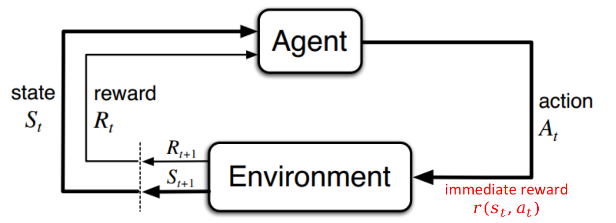
Note: We should be aware of the state reward and state-action reward. See the following figure. In MDP at time $t$, agent is in state $S_t$. When it chooses an action $A_t$, the agent can receive an immediate reward $r(s_t,a_t)$. It is more like the reward on the action. We can compare it with the control cost $u_k^T{u}_k$ in the optimal control. Some literature do not define this immediate reward.

After the agent chooses the action, the environment will respond to it and generate the new state $S_{t+1}$ and the reward $R_{t+1}$. Note that $R_{t+1}$ may not relate to the state and can be completely random. But to simplify the analysis, we assume that the generated reward $R_{t+1}$ is a function of $S_{t+1}$. This means that when the realization of $S_{t+1}$ is determined, the reward $R_{t+1}$ is also determined.

The above argument makes more sense when considering robotic applications. We can use MDP for high level planning. At time $t$, the robot is state $S_t=s$ and it chooses a action $A_t=a$, which gives an immediate action cost $c(s,a)$. After that, the mission status changes to $S_{t+1}=s^{\prime }$. The robot will receive a reward $r(s^{\prime })$ based on the mission status, which can be either good or bad. Therefore, the utility of the robot is simply $u(s^{\prime },s,a)=r(s^{\prime })-c(s,a)$. It is very like the cost in optimal control: $x_{k+1}^T{x}_{k+1}+u_k^T{u}_k$. This shows that the state-reward function is not in the same time step as the state-action reward. This is why in Sutton’s book, the objective of MDP is to maximize $R_{t+1}+\cdots$ while in Filar’s book, the objective is to maximize $R_t+R_{t+1}+\cdots$.

Since MDP is a sequential decision making problem, we denote $S_t$ as the state at time $t$. So is $A_t$, $R_t$. Note that $S_t,A_t,R_t$ are actually random variables. $S_t=s$ and $A_t=a$ are the realizations. The expectation of $R_t$ can be computed by $p$ and $r$.

The transition kernel defines the dynamics of the MDP. It also indicates the environment model. For example, we can define $p(s^{\prime },r|s,a)=Pr[S_{t+1}=s^{\prime },R_{t+1}=r|S_t=s,A_t=a]$, which means the environment is also MDP. See Chapter 3. We can also define state-transition probability $p(s^{\prime }|s,a)=Pr[S_{t+1}=s^{\prime }|S_t=s,A_t=a]$ which is simply $\sum _{r}p(s^{\prime },r|s,a)$. In this way, we assume each state corresponds to a unique immediate reward.

Note: The size of $\mathcal{S}$ usually equals the size of $\mathcal{R}$. The immediate reward does not necessarily corresponds to the current state unless we have a complete information of the environment. For example, at time $t$ we are in $S_t=s$, but the immediate reward does not have to be $R_t=r$. The environment may also do MDP, so there is a probability that the reward is $r$ when we reach state $s$. Usually people consider finite MDP model, which means that the size of $\mathcal{S}$ and $\mathcal{A}$ are finite.

Note: the policy $\pi (a|s)$ is fact stationary. It does not change with the time horizon, which mean we do not have ${\pi }_t(a|s),{\pi }_{t+1}(a|s)$.

We define the return $G_t=R_{t+1}+\gamma R_{t+2}+\cdots =\sum _{k=0}^{\mathrm{\infty }}{\gamma }^k{R}_{t+k+1}$. We also define the state-value function $v_{\pi }(s)={\mathbb{E}}_{\pi }[G_t|S_t=s]$. Note that different policy $\pi$ corresponds to different state-value functions. There is an optimal state-value function, which corresponds to the optimal policy ${\pi }^{\ast }$.

The objective of MDP is to find the optimal policy ${\pi }^{\ast }$ such that the expected return $\mathbb{E}[G_t|S_t=s]$ is maximized. The corresponding state-value function is denoted as $v_{\pi }^{\ast }(s)$.

We derive the fundamental property of state-value functions which is similar to DP.

The first term tells

The summation is over $s^{\prime }$ because we assume the reward and state has one-to-one correspondence. We denote the reward as $r_{s^{\prime }}$. The second term tells

Therefore, putting them together, we have

Solution and algorithm

value iteration, policy iteration, LP: 15-780: Markov Decision Processes