Markov Decision Processes

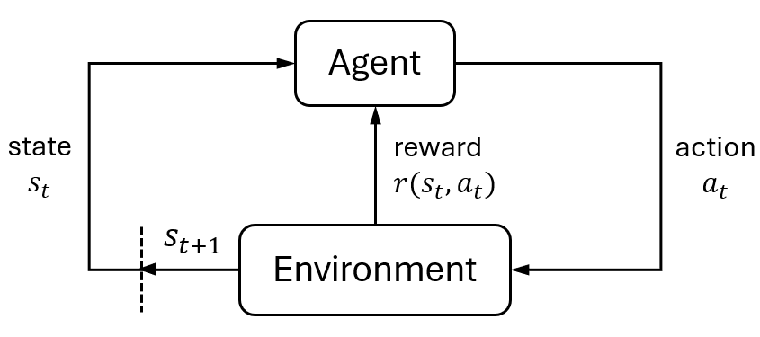
The Markov decision process (MDP) is a mathematical framework for making sequential decisions under uncertainty¹. It models how an intelligent agent selects actions to transition between states and accumulate corresponding rewards. The ultimate goal of the agent is to find the optimal policy—a strategy that dictates the best action to take in each state—to maximize the total reward over time.

A motivating example is the decision-making process in a student’s study journey.

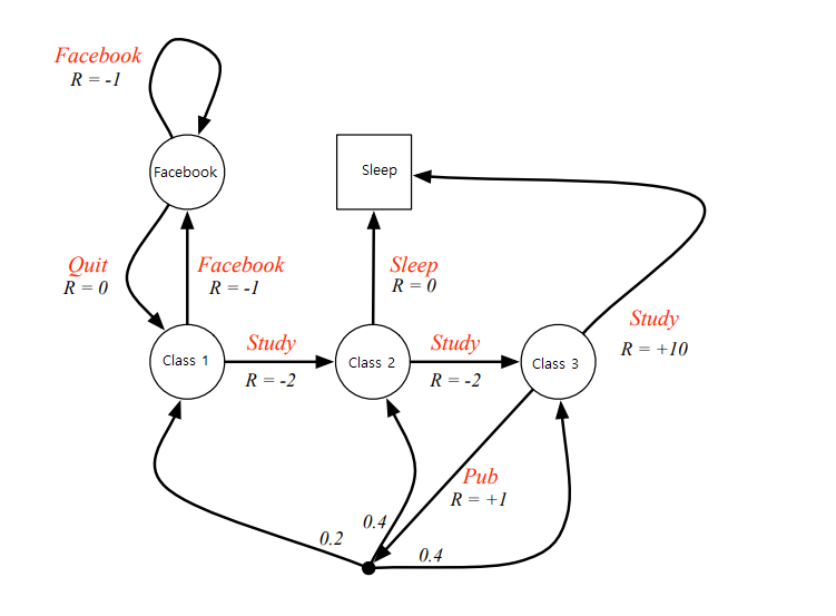
In this scenario, states such as “sleep” or “class 1” represent different stages in the student’s learning process. From a given state—say, “class 1”—the student can choose an action like “study,” which may lead to another state like “class 2.” Each action yields a reward, typically represented by a score. The student’s objective is to develop a plan, or policy , that maximizes the cumulative reward throughout the learning process.

This kind of sequential decision-making can be naturally modeled using an MDP. MDPs provide a simple yet powerful abstraction that captures how agents interact with their environment and how the environment evolves in response. They also form the foundation of reinforcement learning (RL) (see Introduction to RL).

Below, we present the formal mathematical formulation of MDPs.

Mathematical Formulation

Intuitively, an MDP extends the concept of a Markov chain (see Markov Chain) by incorporating actions and rewards. Formally, it is defined by the tuple $\langle \mathcal{S}, \mathcal{A}, T, r, \gamma \rangle$, where

• $\mathcal{S}$: the set of all possible states. We denote a particular state by $s$.
• $\mathcal{A}$: the set of all possible actions. We denote a specific action by $a$.
• $T: \mathcal{S} \times \mathcal{A} \times \mathcal{S} \to [0,1]$: the transition kernel, defined as the conditional probability $p(s’ \vert s, a)$, representing the likelihood of transitioning to state $s’$ after taking action $a$ in state $s$.
• $r: \mathcal{S} \times \mathcal{A} \to \mathbb{R}$: the reward function denoted by $r(s,a)$, which returns the immediate scalar reward after taking action $a$ in state $s$.
• $\gamma \in [0,1]$: the discounted factor, which determines the present value of future rewards.

Some important points to note:

• MDPs satisfy the Markov property: the next state depends only on the current state and action, not on the history of previous states or actions.
• States and actions can be either discrete or continuous, leading to discrete or continuous MDPs. Here, we discuss discrete MDPs, which are the most commonly stuided.
• Some literature (e.g., Sutton² ) define a state-action-state reward function $r(s,a,s’)$ to consider the transition effect. In that case, we have $r(s,a) = \sum_{s’} p(s’ \vert s,a)r(s,a,s’)$.

Probabilistic Transition Kernel

The transition kernel models the dynamics of the environment. There are two main reasons why transitions are often modeled probabilistically:

1. Generality : Probabilistic transitions generalize deterministic ones. Thus, even environments with deterministic dynamics, such as vehicle navigation systems, can be modeled using MDPs.
2. Computational convenience : Probabilistic formulations allow us to use continuous optimization techniques rather than treating the problem as combinatorial.

Under this probabilistic model, let random variables $S$ and $A$ represent the current state and action, respectively. Then the transition kernel is defined as

Policy and Objective

A policy is a function to generate actions in some state. Here, it is defined as $\pi(a \vert s)$, which is a probability distribution over actions for each state, so that $\sum_a \pi(a\vert s) = 1$. Let $\Pi$ denote the set of all feasible policies.

The objective of an MDP is to find a policy $\pi$ that maximizes the expected cumulative reward over time, which is

Here,

1. $S_t, A_t$ are random variables representing the state and action at time $t$.
2. The initial state $S_0$ can be a fixed value $s$ or drawn from an initial distribution $\rho$.
3. The discounted factor $\gamma$ ensures that the infinite sum remains finite.

Depending on applications, several variants of this objective exist:

• Finite-horizon MDP: Limits the decision horizon to the finite length.

• Averaging MPD: Focuses on the long-term average reward per step.

We explore solution methods for these variants in separate discussions.

Finite-Horizon vs Infinite-Horizon (other posts…)

The decision horizon $T$, in fact, plays an important role in shaping the optimal policy of \eqref{eq:mdp}. If $T = \infty$, the optimal policy $\pi^\ast$ is stationary; if $T < \infty$, the optimal policy is nonstationary, meaning that we have different $\pi^*$ at each time, denoted by $\boldsymbol{\pi}^\ast = [ \pi^\ast_0, \pi^\ast_1, \dots, \pi^\ast_{T-1} ]$. The short explanation is that as $T \to \infty$, the MDP does not differentiate time steps since we will always solve the same MDP starting from any $t$. Thus, the policy is the same.

Infinite-horizon MDPs are common for researchers due to stationary policies. Note that if $T = \infty$, we need $\gamma < 1$ to ensure the accumulated reward is bounded.

MDP finite horizon (other posts…)

dp principles, derivation

MDP avaraging reward infinite horizon (other posts…)

solution methods, derivation

Value Functions

Value functions play a central role in solving MDPs. Their properties form the foundation of many solution methods used to find optimal policies. Two key types of value functions are:

• The $V$-function, or state-value function, which evaluates the expected cumulative reward starting from a given state under a specific policy.
• The $Q$-function, or action-value function. which evaluates the expected cumulative reward starting from a given state-action pair under a policy.

Below, we define and explore these functions for infinite-horizon MDPs. These definitions can be adapted to finite-horizon settings as well.

$V$-Function

The objective of an MDP is given by an infinite series. To simplify this, we introduce the value $v^\pi(s)$ as the expected total discounted reward starting from state s and following policy $\pi$ thereafter:

We can derive a recursive relationship for $v^\pi(s)$ using a one-step expansion:

The second expectation term starts from $t=1$ and $S_1$ is a random variable. Since the random action $A_0$ is processed in the first term, the second term is eaiser to understand by writing it as \(\mathbf{E}_{p,\pi} \left[ \sum_{t=1}^\infty \gamma^t r(S_t, A_t) \vert S_1 \sim \rho' \right]\) for some distribution $\rho’$. Since we start from $S_0=s$, the probability of reaching an arbitrary state $S_1=s_1$ is $\sum_{a} \pi(a\vert s) p(s’\vert s, a) := \rho’(s’)$. Assume $S_1 = s’$ is given, we have

because of the infinite summation. Considering all possible $s_1$, we arrive at

Equation \eqref{eq:bellman-v} is known as the Bellam equation for the $V$-function. This recursive structure allows us to compute the value function iteratively. We define the Bellman operator $B: \mathbb{R}^{\vert \mathcal{S} \vert} \to \mathbb{R}^{\vert \mathcal{S} \vert}$, which maps a value vector to another via the bellman update

Therefore, the vaule function $\boldsymbol{v}^\pi$ satisfies a fixed-point equation

Because the Bellman operator is a contraction mapping³, we can compute $\boldsymbol{v}^\pi$ either by solving a linear system or through iterative updates such as

This forms the basis of many dynamic programming algorithms.

$Q$-Fucntion

While the $V$-function evaluates the expected return from a state, the $Q$-function evaluates it from a state-action pair. This distinction becomes especially important when evaluating or improving policies, since the optimal policy often selects actions greedily based on the $Q$-value (discussed in Properties of Optimal Policy).

We define the $Q$-function under policy $\pi$ as

There is a direct relationship between the $V$-function and the $Q$-function:

Following a similar derivation, we obtain the Bellman equation for the $Q$-function:

Just like with the $V$-function, we can define the corresponding Bellman operator and uses fixed-point iteration to compute the $Q$-function under any given policy.

Note that the $Q$-function is particularly useful in model-free reinforcement learning, where knowledge of the environment dynamics $p(s’\vert s,a)$ is not required.

Properties of Optimal Policy

The Bellman equations \eqref{eq:bellman-v} and \eqref{eq:bellman-q} hold for any feasible policy $\pi$, including the optimal policy $\pi^\ast$. It is a well-known result that for infinite-horizon MDPs, optimal policy $\pi^\ast$ is stationary and deterministic (Filar, Chap:2.3⁴). That is, $\pi^\ast(a\vert s)$ assigns full probability mass to a single action for each state.

Under the optimal policy, The bellman equation becomes

Furthermore, the optimal $V$-function is related to the optimal $Q$-function by:

Equations \eqref{eq:bellman-vstar} and \eqref{eq:bellman-qstar} are at the heart of many MDP solution algorithms, including value iteration and policy iteration.

Solution Methods

For discrete MDPs, solution methods are often referred to as tabular methods, because the $V$- and $Q$-functions can be represented as $\vert \mathcal{S} \vert \times 1$ and $\vert \mathcal{S} \vert \times \vert \mathcal{A} \vert$ tables, respectively.

Solution methods fall into two main categories:

• Mathematical programming: Formulates the problem as an optimization task.
• Iterative methods: Uses the Bellman operator iteratively to converge to the optimal value function.

Among iterative methods, common approaches include policy iteration, value iteraion, multistage lookahead policy iteration, and $\lambda$-policy iteration.

Linear Programming

Linear programming approach directly uses the Bellman equation \eqref{eq:bellman-vstar}. It treats the elements of $V$-functions as decision variables and solves the following LP:

Here, $\rho$ denotes the initial state distribution. A special example is $\rho \sim \operatorname{Uniform}$, which produces $\sum_s \rho(s) v(s) = \frac{1}{\vert \mathcal{S} \vert} \sum_s v(s)$. This formulation has $\vert \mathcal{S} \vert$ decision variables and $\vert \mathcal{S} \vert \times \vert \mathcal{A} \vert$ constraints. Each constraint upper bound the value function based on the Bellman equation, with equality holding only for optimal actions. Once the optimal value function $v^*$ is obtained, the optimal policy is recovered via:

We can find the dual problem of the primal LP \eqref{eq:primal}, which is

The dual problem is interesting because it produces many important results.

1. Let $\pi$ be a feasible policy of the MDP and $\rho$ be the initial state distribution. We define the occupancy measure

which measures the culmulative probability of the event $S_t=s,A_t=a$. We can verify that $\nu^\pi$ is a feasible solution of the dual LP \eqref{eq:dual}.

2.Suppose $\mu(s,a)$ is a feasible solution of the dual LP \eqref{eq:dual}. Then for each $s \in \mathcal{S}$ such that $\sum_a \mu(s,a) > 0$, we can induce a stationary policy $\pi_\mu$ by

Then, the occupancy measure $\nu_{\pi_\mu}$ induce by $\pi_\mu$ is equal to $\mu$. i.e., $\mu(s,a) = \nu_{\pi_\mu}(s,a)$ for all $s \in \mathcal{S}$ and $a \in \mathcal{A}$.

3.If $\mu^\ast$ is the optimal solution of the dual LP \eqref{eq:dual}, then the induced policy $\pi_{\mu^\ast}$ is the optimal solution of the primal LP \eqref{eq:primal}. Besides, $\pi_{\mu^\ast}$ is deterministic.

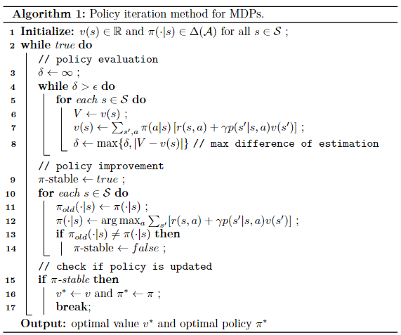
Policy Iteration

Policy iteration is the most typical method in iterative methods. It iteratively run the two processes: policy evaluation and policy improvement, to find the optimal policy and the optimal value function. Specifically,

In the policy evaluation (also called prediction):

• compute the value function $v^\pi(s)$ or $q^\pi(s,a)$ using the current policy $\pi$.
• solve a linear system $v=B(v)$ or $q = B(q)$.

In the policy improvement (also called update):

• generate a new policy $\pi’$ using the current vaule function $v^\pi(s)$ or $q^\pi(s,a)$.
• greedy maximization (most common)

Other iterative methods follow the same two processes but differ in the policy evaluation process. We summarize the policy iteration algorithm in Fig. 3.

Convergence? change iteration to $k$ in alg?

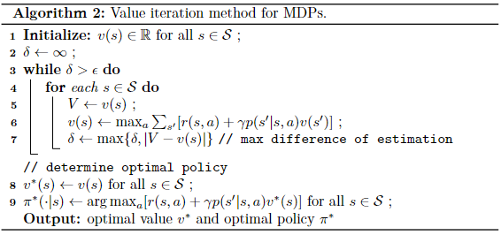
Value Iteration

Value iteration is a special case of policy iteration. It updates the value function only once in the policy evaluation process instead of computing the real $v^\pi$. This operation is more concise when $\mathcal{S}$ is large because policy iteration needs to run an iterative loop for every state to obtain the value $v^\pi(s)$. However, the drawback of value iteration is that it may converge very slowly. This is true for many problems with large state space or with a discounted factor $\lambda$ close to 1.

v-funciton, q funciton.

convergence? change iteration to $k$ in alg?

Multistage Lookahead Policy Iteration

As we observe, when the state space is large, policy iteration methods will take a lot of time in the policy evaluation process, the for loop is terminated when the difference is smaller than a threshold. Although value iteration only evaluate one-step policy evaluation, it converges slowly. Therefore, a balance is to use a fixed step evaluation $m > 1$ in the policy evaluation process. which improves the convergence. The rest remains the same.

$\lambda$-Policy Iteration

unifies two methods³. reduce the discounted factor to achieve faster decay, especially useful for large $\gamma$. The policy evaluation is different, changes to $v_{k+1} = v_k + \Delta_k$, where $\Delta_k \in \mathbb{R}^{\vert \mathcal{S} \vert}$ is the value vector of a $\gamma \lambda$-discounted MDP problem with transition probabilities $p^{\pi_{k+1}} = \sum_a \pi_{k+1}(a \vert s) p(s’ \vert s,a)$.

where $d_k$ is the temporal difference at step $k$ under policy $\pi_{k+1}$

Computing $\Delta_k$ is not hard, same as iteration in policy iteration methods. We can also compute $m$ terms of $\Delta_k$ for approximation.

When $\lambda=0$, we have value iteration, when $\lambda=1$, we have policy iteration. When use iteration with $\lambda < 1$, policy evaluation converges faster compared with $\lambda=1$. However, small $\lambda$ does not perform well.

convergence? alg?

We should note that only PI compute $v^{\pi_k}$ given $\pi_k$. value iteration and multi-step lookahead, $\lambda$-policy with $\lambda < 1$ all finds an approximate value, i.e., $v_k$ not $v^{\pi_k}$.

Short Summary

We have introduced the formulation, value functions, and solution methods for infinite-horizon Markov Decision Processes (MDPs). MDPs provide a general and powerful framework for sequential decision-making under uncertainty, and have enabled impactful applications across various domains, including robotics, transportation, and communication systems. Although domain-specific knowledge is often required to model real-world problems as MDPs, the underlying solution methods remain consistent across fields.

MDPs also have several variants. For example, finite-horizon MDPs are useful when decisions are made over a fixed time horizon, while average-reward MDPs are suitable for long-run average performance criteria. These variants extend the applicability of the framework to different types of sequential decision problems.

Recommended References

For a comprehensive and rigorous treatment of MDPs, including both discrete and continuous formulations, we highly recommend the textbook by Puterman¹ and Filar⁴.

For an accessible introduction from a reinforcement learning perspective, Prof. Silver’s Lectures Slides on Reinforcement Learning⁵ and Prof. Kolter’s slides on MDPs⁶ would be a good starting point.