Continuous Randon Variables

Probability mass functions

Definition 1. The (probability) mass function (p.m.f.) of a discrete random variable $X$ is the function $f : R \to [0, 1]$ given by $f (x) = P (X = x)$ .

Notice that $f (x)$ is not discontinuous. The distribution and mass functions are related by $F (x) = \sum_{i : x_{i} \leq x} f (x_{i}), f (x) = F (x) - lim_{y ↑ x} F (y) .$

Lemma. The probability mass function $f : R \to [0, 1]$ satisfies:

the set of $x$ such that $f (x) \neq 0$ is countable,
$\sum_{i} f (x_{i}) = 1$ , where $x_{1}, x_{2}, \dots$ are the values of $x$ such that $f (x) \neq 0$ .

Example. Binomial distribution. A coin is tossed $n$ times, and a head turns up each time with probability $p (= 1 - q)$ . Then $Ω = {H, T}^{n}}$ . The total number $X$ of heads takes values in the set ${0, 1, 2, \dots, n}$ and is a discrete random variable. Its probability mass function $f (x) = P (X = x)$ satisfies $f (k) = (\binom{n}{k}) p^{k} (1 - p)^{n - k}, k = 0, 1, \dots, n .$ The random variable $X$ is said to have the binomial distribution with parameters $n$ and $p$ , It is the sum $X = Y_{1} + Y_{2} + \dots + Y_{n}$ of $n$ Bernoulli variables.

Example. Poisson distribution. If a random variable $X$ takes values in the set ${O, 1, 2, \dots}$ with mass function $f (k) = \frac{λ^{k}}{k!} e^{- λ}, k = 0, 1, 2, \dots,$ where $λ > 0$ , then $X$ is said to have the Poisson distribution with parameter $λ$ . Figure 1. shows how p.m.f varies with $k$ .

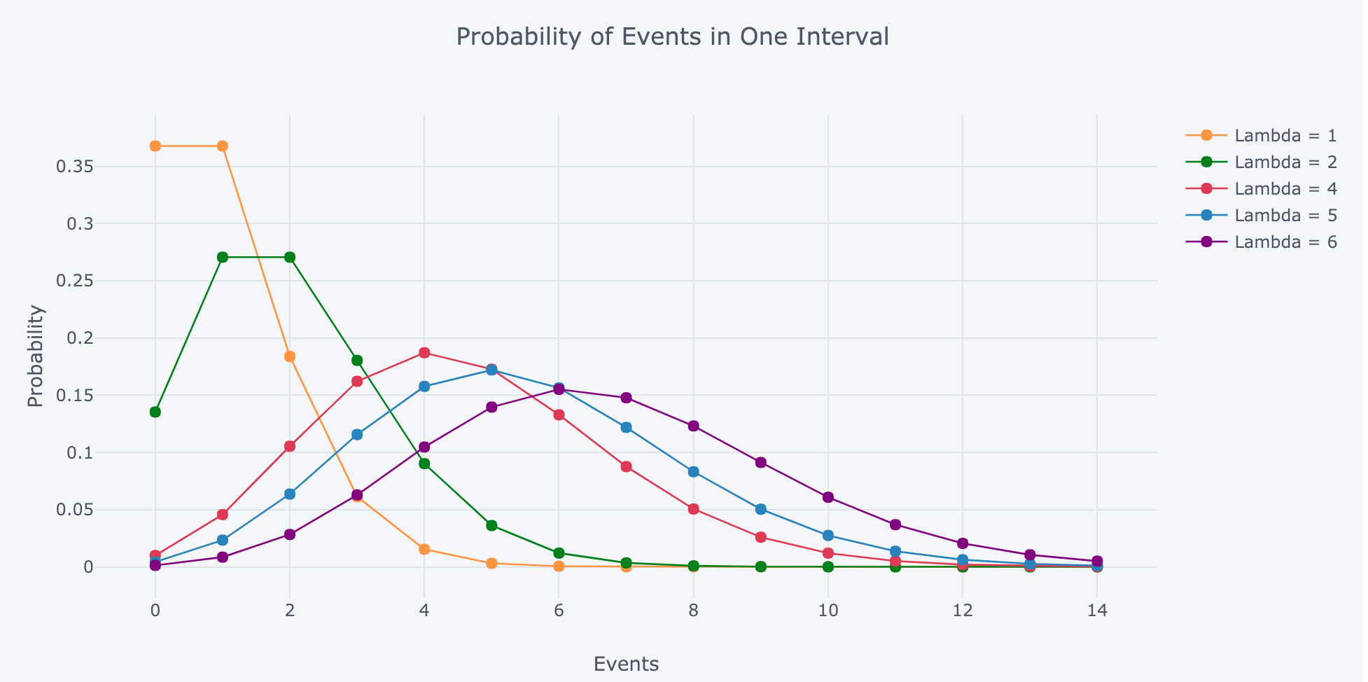
Remark. The interpretation of Poisson distribution can be found via this link: The Poisson Distribution and Poisson Process Explained.

Independence of discrete random variables

Recall that events $A$ and $B$ are called independent if and only if $P (A \cap B) = P (A) P (B)$ .

Definition 2. Discrete variables $X$ and $Y$ are independent if the events ${X = x}$ and ${Y = y}$ are independent for all $x$ and $y$ .

Let $A := ω | X (ω) = x$ and $B := ω | Y (ω) = y$ . Then we can write $P (A) = f_{X} (x), P (B) = f_{Y} (y)$ and $P (A \cap B) = f (x, y)$ . Therefore, $A$ and $B$ are independent if and only if $f (x, y) = f_{X} (x) f_{Y} (y)$ for all $x$ and $y$ .

Remark. The equality $f (x, y) = f_{X} (x) f_{Y} (y)$ can be used as the criterion to determine whether two discrete random variables $X$ and $Y$ are independent or not. But we need to be careful with it when dealing with continuous random variables as there will be additional assumptions to determine the independence of continuous random variables using this equality.

Theorem 1. If $X$ and $Y$ are independent and $g, h : R \to R$ , then $g (X)$ and $h (Y)$ are independent also.

More generally, we say that a family $X_{i} | i \in I$ of (discrete) random variables is independent if the events $X_{i} = x_{i}, i \in I$ , are independent for all possible choices of the set $x_{i} | i \in I$ of the values of the $X_{i}$ . That is to say, $X_{i} | i \in I$ is an independent family if and only if $P (X_{i} = x_{i} for all i \in J) = \prod_{i \in J} P (X_{i} = x_{i})$ for all sets $x_{i} | i \in I$ and for all finite subsets $J$ of $I$ .

Probability density functions

Recall that a random variable $X$ is continuous if its distribution function $F (x) = P (X \leq x)$ can be written as\footnote{This is just a general integral, $f (u)$ may or may not be continuous.} $F (x) = \int_{\infty}^{x} f (u) d u$ for some integrable $f : R \to [0, \infty)$ .

Definition 3. The function $f$ is called the (probability) density function (p.d.f.) of the continuous random variable $X$ .

Remark. The function $f$ is NOT unique. We can add some separate points or a countable set of points which has zero measure to $f$ . This doesn't change the value of the integral. However, if $F$ is differentiable at $u$ then we shall normally set $f (u) = F^{'} (u)$ .

Next, we assume $f$ is continuous, then from the basic theorem of calculus, $F$ must be differentiable. Recall $P (a < X (ω) \leq b) = F (b) - F (a) = \int_{a}^{b} f (u) d u .$ Then $P (X = x) = F (x) - lim_{y ↑ x} F (y)$ . $F$ is absolutely continuous for continuous random variables. Thus we have $lim_{y ↑ x} F (y) = F (x) R i g h t a r r o w P (X = x) = 0 \forall x \in R .$ This means the probability of a continuous random variable $X$ taking value at a certain point is 0. Very roughly speaking, this lies in the observation that there are uncountably many possible values for $X$ ; this number is so large that the probability of $X$ taking any particular value cannot exceed zero.

The numerical value $f (x)$ is NOT a probability. Check the probability $P (x < X \leq x + d x)$ for a very small $d x$ : $P (x < X \leq x + d x) = F (x + d x) - F (x) \approx f (x) d x .$ Since $d x$ is a very small interval rather a number, we cannot say $f (x)$ is the probability of something.

Lemma. If $X$ has density function $f$ , then

$\int_{- \infty}^{\infty} f (x) d x = 1$ ,
$P (X = x) = 0$ for all $x \in R$ ,
$P (a < X \leq b) = \int_{a}^{b} f (x) d x$ .

Independence of continuous random variables

Independence of general random variables

Definition 4. Random variables $X$ and $Y$ are called independent if ${X \leq x}$ and ${Y \leq y}$ are independent events for all $x, y \in R$ .

Note that this definition is the general definition of the independence of any two variables $X$ and $Y$ regardless of their types. The independence of discrete random variables is included in this definition.

Recall the marginalization. If two random variables $X$ and $Y$ are independent, we have $P (X \leq x) = lim_{y \to \infty} F (x, y) \equiv F_{X} (x), P (Y \leq y) = lim_{x \to \infty} F (x, y) \equiv F_{Y} (y) .$ Therefore, $\begin{matrix} (1) & F (x, y) = P (X \leq x, Y \leq y) = P (X \leq x) P (Y \leq y) = F_{X} (x) F_{Y} (y) . \end{matrix}$ Note that we are dealing with distribution function in Eq.(1). Eq.(1) can be used as the general criterion to determine whether two random variables are independent or not.

Independence of continuous variables

If $X, Y$ are continuous, then we have $F (x, y) = \int_{- \infty}^{x} \int_{- \infty}^{y} f (x, y) d x d y .$ $F_{X} (x) = \int_{- \infty}^{x} \int_{- \infty}^{\infty} f (x, y) d x d y R i g h t a r r o w f_{X} (x) = \int_{- \infty}^{\infty} f (x, y) d y,$ where $f_{X} (x)$ is called the marginal probability density function of $X$ . Similarly, we can define $F_{Y} (y)$ and $f_{Y} (y)$ .

Assume $f (x, y)$ is continuous, then $F (x, y)$ must be twice differentiable w.r.t. $x$ and $y$ . Therefore, from \eqref{eq:}, we can derive a *very practical criterion to determine the independence of two continuous random variables: $\begin{matrix} (2) & f (x, y) = \frac{\partial^{2} F (x, y)}{\partial x \partial y} = \frac{\partial}{\partial x \partial y} F_{X} (x) F_{Y} (y) = f_{X} (x) f_{Y} (y) . \end{matrix}$

Remark. Note that the prerequisite of Eq.(2) is that $f (x, y)$ is continuous.

Example. Uniform distribution. The random variable $X$ is uniform on $[a, b]$ if it has distribution function $F (x) = {\begin{cases} 0 & x \leq x, \\ \frac{x - a}{b - a} & a < x \leq b, \\ 1 & x > b \end{cases} .$ The density function is $f (x) = {\begin{cases} \frac{1}{b - a} & a < x \leq b \\ 0 & o . w . \end{cases}$

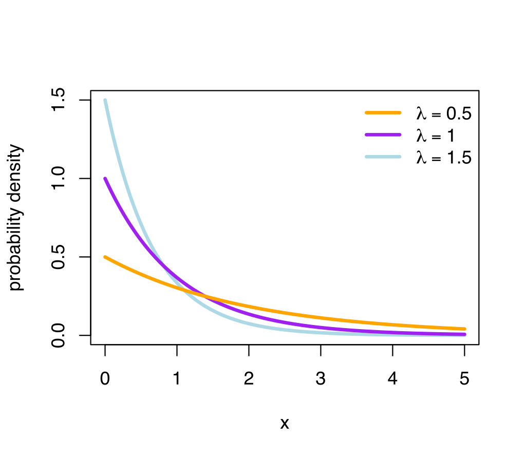
Example. Exponential distribution. The random variable $X$ is exponential with parameter $λ (> 0)$ if it has distribution function $F (x) = 1 - e^{- λ x}, x \geq 0.$ The density function is $f (x) = {\begin{cases} λ e^{- λ x} & x > 0 \\ 0 & o . w . \end{cases}$ Note that $F (x)$ is not differentiable at $x = 0$ . This means $f$ has discontinuity at $x = 0$ . Thus we need to choose some value for $f (0)$ . It doesn't matter what value we choose as it doesn't affect the integral. Figure 2 shows the p.d.f. of Exponential distribution.

Fig.2: p.m.f of exponential distribution.

Remark. The interpretation of Exponential distribution can be found via Exponential distribution 1 and Exponential distribution 2. Pay attention to the connection between Exponential distribution and Poisson distribution.

Example. Normal (or Gaussian) distribution. The most important continuous distribution, which has two parameters $μ$ and $σ^{2}$ and density function $f (x) = \frac{1}{\sqrt{2 π σ^{2}}} \exp (- \frac{(x - μ)^{2}}{2 σ^{2}}), x \in R .$ It is denoted by $N (μ, σ^{2})$ . If $μ = 0$ and $σ^{2} = 1$ , then $f (x) = \frac{1}{\sqrt{2 π}} e^{- \frac{1}{2} x^{2}}, x \in R .$ is the density of the standard normal distribution. It is easy to generalize 2D case to multivariable case. Suppose $x \in R^{n}$ , $μ \in R^{n}$ is the mean vector and $σ^{2} \in R^{n \times n}$ is the covariance matrix. Then $f (x) = \frac{1}{\sqrt{(2 π)^{n}} det (σ^{2})} \exp (- \frac{1}{2} (x - μ)^{T} (σ^{2})^{- 1} (x - μ)), x \in R^{n} .$

Remark. For 2D case, if $σ^{2}$ is diagonal, then $f (x, y) = f (x) f (y)$ . Therefore, $σ^{2}$ is a measure of independence. For multivariable cases, if $σ^{2}$ is diagonal, then all random variables are independent with each other.